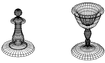

Viewing and manipulating models of three-dimensional objects is a common task in sophisticated graphics packages. We will only be able to introduce some of the most basic concepts of 3-D modeling in the short time we have left in this course. In particular, we will look at how to create wireframe and polygon mesh models of three-dimensional objects, how to view these models in a two-dimensional graphics window, and how to apply basic scene transformations (scaling, translation, and rotation).
Table of Contents:
Imagine, for a moment, that you want to build a physical model of a cube. One reasonable approach would be to cut six squares of the same size and tape them together to form a cube. A slightly better approach might be to cut out the following T-shaped pattern, fold along the dotted lines, and tape common edges together to form a cube.

Both of these approaches would result in a physical model based on reproducing the faces of the cube (the edges and vertices are created only as a byproduct of creating the faces):

Another approach to making a physical model of a cube would be to focus on creating the edges rather than the faces. Cut 12 pieces of wire exactly the same length and solder the ends together to create the model:

While this second approach is harder in the real world, it is much easier in the digital world. A wireframe model consists of a list of vertex coordinates and a list of edges. Each edge is represented by its endpoints. Here is an example file (where the text is not actually part of the file):
8              The number of vertices
1 1 1          Vertex 1
-1 1 1         Vertex 2
-1 -1 1
1 -1 1
1 1 -1
-1 1 -1
-1 -1 -1
1 -1 -1        Vertex 8
12             The number of edges
1 2            Edge from vertex 1 to vertex 2
1 4            Edge from vertex 1 to vertex 4
1 5
2 3
2 6
3 4
3 7
4 8
5 6
5 8
6 7
7 8            Edge from vertex 7 to vertex 8
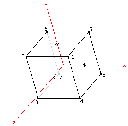
As you may have already discovered, wireframe models can be somewhat difficult to interpret since you can see right through them. In the image above, I colored the edges that would not be visible in a solid model, a light gray. In our application we will not be able to do that.
We will be viewing our models straight down the z-axis. Conceptually, imagine our wireframe model suspended in space just above a piece of paper placed on a horizontal surface. Now imagine that there is a bright light (such as the sun) directly overhead but at an infinite distance. All of the light beams coming from this light are parallel to each other and the shadow of the object on the paper is a parallel projection of a 3-D object onto a 2-D plane. In effect, the 2-D image is obtained by plotting only the x- and y- coordinates of the vertices and ignoring the z coordinates (in effect, setting the z-coordinates to zero). This is also referred to as an orthogonal or orthographic projection.
An orthogonal projection ignores the fact that in the real world the farther away an object is, the smaller it will appear to be. Given two identical sized objects, the closer one will appear larger than the one that is farther away. A perspective projection takes this change in apparent size into account and in some cases, makes it a little easier to determine the orientation of an object.
Consider something as simple as our cube model (centered on the origin). Viewed straight down the z-axis using an orthogonal projection, the cube looks like a square (see the left side of the image below). Using a perspective projection, the front face is a little bigger than it was because it is closer to us than the xy-plane. The rear face is a little smaller than before because the rear face is behind the xy-plane. The edges joining the two faces appear as short diagonal lines:

The larger an object is, the more pronounced the difference between an orthogonal and perspective projection:
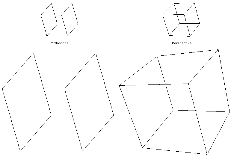
In a perspective projection, the light comes from a point source at a relatively short distance above the xy-plane (our imaginary piece of paper). Consequently the light beams emanating from the light fan out in all directions from the light source to the xy-plane. As a result, the shadow of items close to the light will appear larger than the shadows of items farther from the light.
In practice, the difference between the x-coordinate and the projected x-coordinate is proportional to the x-coordinate and the constant of proportionality is some percentage of the corresponding z-coordinate. The same is true for the y-coordinate:
Δx = kx where k = pz
x + Δx = x + (pz)x = x(1 + pz)

Δy = ky where k = pz
y + Δy = y + pzy = y(1 + pz)
Increasing the percentage, p, makes the perspective effect more pronounced and decreasing the percentage makes it less pronounced. If the z-coordinate is positive, the projected x- and y-coordinates will be further from the origin than the actual coordinates. If the z-coordinate is negative, the projected points will be closer to the origin. In either case, the larger the magnitude of the z-coordinate, the more pronounced the effect.
In a similar fashion, increasing the percentage is equivalent to moving the light closer to the plane and the perspective effect will be enhanced. Decreasing the percentage is equivalent to moving the light further from the plane and the perspective effect will be diminished.
Conceptually, viewing the scene from different vantage points can be thought of in two different ways. One approach is to think of the scene as fixed in space while the observer is free to move around. The second is to think of the observer as fixed in space while the scene is free to move around.
Consider our basic cube and suppose we are looking at the cube from straight down the z-axis with the xy-plane oriented in the normal way (x to the right and y up). Suppose we want to view the same object from straight down the x-axis. One approach would be for us to move around until we are looking at the scene down the x-axis. The other approach would be to stay where we are and rotate the model until we are looking down the x-axis. The two approaches are illustrated below (where we are looking down on the observer and the scene along the y-axis).
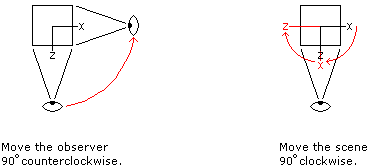
We will be using the second approach in which the scene is manipulated and the observer remains stationary.
A scaling transformation changes the apparent size of the scene. A scaling transformation involves multiplying each coordinate of a point by a scaling factor:
xnew = sx * xold
ynew = sy * yold
znew = sz * zold
If the scaling factors are all the same, the relative dimensions will be preserved. If the scaling factors are different, the scene will be stretched (or shrunk) more in some directions than in others.
Translating a scene means moving the scene to a new location. Translation occurs along one or more of the axes. When viewed down the z-axis, movement along the x-axis will appear as movement left or right. Movement along the y-axis will appear as movement up or down. Movement along the z-axis will bring the scene closer to the observer or farther away. (Movement along the z-axis is not apparent if an orthogonal projection is being used but will be apparent if a perspective projection is being used to display the image.)
A translation transformation involves adding a translation distance to each coordinate of a point:
xnew = xold + tx
ynew = yold + ty
znew = zold + tz
The translation distance corresponds to the distance the scene will be moved along the corresponding axis.
The scene can be rotated about any of the three axes. A positive angle of rotation corresponds to a counterclockwise rotation as viewed along the positive axis. A positive rotation about the x-axis will be a rotation from the y-axis towards the z-axis. A positive rotation about the y-axis is a rotation from the z-axis toward the x-axis. A rotation about the z-axis is a rotation from the x-axis towards the y-axis.
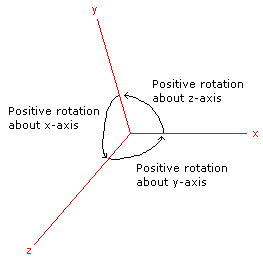
A rotation transformation is significantly more complicated than either a scaling transformation or a translation transformation. Let's consider a positive rotation of θ about the z-axis from point (x, y) to point (x', y'):
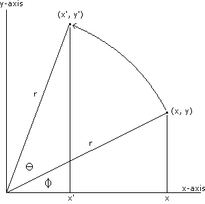

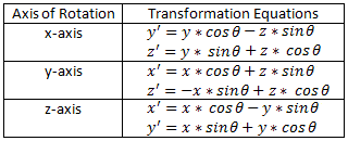
The rotation transformations for rotation about the x-axis and a rotation about the y-axis are derived in a similar fashion. The results are summarized in the table below. Notice that in each case, the variable along the axis of rotation is not changed. For example, when rotating about the x-axis, the value of x is not changed; just the values of y and z.
Mathematically, each transformation described above can be written as a 4 x 4 matrix (T) and each point can be written as a 4 x 1 matrix (P). The product of a transformation matrix and a point matrix yields the matrix representation of the new point (P' = TP).
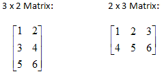
A matrix is a two-dimensional table of numbers whose size is specified by the number of rows and the number of columns. For example, a 3 x 2 matrix has 3 rows and 2 columns and a 2 x 3 matrix has 2 rows and 3 columns:
In essence, a matrix is just a two-dimensional array with some special mathematical properties.
Matrix multiplication is defined for two matrices if the number of columns in the first (left) operand is equal to the number of rows in the second (right) operand. The product has the same number of rows as the first operand and the same number of columns as the second:

We'll begin with multiplying a row matrix by a column matrix:

Observe that matrix multiplication is defined for a 1 x n and a n x 1 matrix because the number of columns in the left operand is the same as the number of rows in the second. Furthermore, the product will be a 1 x 1 matrix. In general, the product of a row matrix by a column matrix is found by multiplying the corresponding values in the two matrices and adding the results. Let R and C represent the row and column matrices and let P represent the product (P = RC). The only value in the 1 x 1 product P is given by:
P1,1 = R1,1 * C1,1 + R1,2 * C2,1 + R1,3 * C3,1 + ... + R1,n * Cn,1
For our specific example given above,

In general, each element in a product matrix is found by multiplying the corresponding row matrix in the left operand by the corresponding column matrix in the second operand:
Pi,j = Rowi * Colj = Ri,1 * C1,j + Ri,2 * C2,j + Ri,3 * C3,j + ... + Ri,n * Cn,j
Here is one example:

Here is another example:

Notice that, unlike ordinary multiplication, matrix multiplication is not commutative. In general, AB ≠ BA. As a matter of fact, in general, if A can be multiplied by B (AB is defined), B cannot be multiplied by A (BA is not even defined). Suppose A is a m x n matrix and B is a n x p matrix. Multiplication is defined for AB but not for BA:
A (m x n) times B (n x p) is defined and the product will be m x p.
B (n x p) times A (m x n) is not defined.
While matrix multiplication may not be commutative, it is associative: ABC = (AB)C = A(BC). As we will see this is a very useful property.
A point in three-dimensional space can be represented as a 4 x 1 matrix whose rows correspond to x, y, z, and 1:
![]()
A scaling transformation matrix is a 4 x 4 matrix of the following form:

The scaling factors sx, sy, and sz are applied to the x, y, and z coordinates as illustrated below. Typically, all three factors are the same so the scaling is the same in all three dimensions. Otherwise, the three-dimensional model will be distorted. The transformed point is found by finding the matrix product of the transformation matrix and the point matrix:

A translation transformation matrix is a 4 x 4 matrix of the following form:

The corresponding translation distance is added to the value of the x, y, and z coordinates as illustrated below. Typically, the three distances are not the same. The transformed point is found by finding the matrix product of the transformation matrix and the point matrix:

A rotation transformation matrix is a 4 x 4 matrix of one of the following forms:
| Rotation about x-axis | Rotation about y-axis | Rotation about z-axis |
 |
 |
 |
In each case, the new point is found by finding the matrix product of the transformation matrix and the point matrix:
| About x-axis |
 |
| About y-axis |
 |
| About z-axis |
 |
In most cases, multiple transformations are applied to a model. For example, suppose we start with a basic cube model, scale it by a factor of 0.5, move it one-half unit in the x-direction, rotate it about the x-axis by -30 degrees, and rotate it about the y-axis by 30 degrees. Let P represent the current point, and let P' represent the new (transformed) point. Furthermore, let S, T, Rx, and Ry represent the transformation matrices. The new point is the result of the following matrix multiplication:
P' = Ry * Rx * T * S * P
Each vertex in the model is
Notice that each transformation is applied to the result of the previous translation. That is, it is the scaled point that is translated, it is the translated, scaled point that is rotated about the x-axis and it is the rotated, translated, scaled point that is rotated about the y-axis. As noted above, the translations must be applied in this order to achieve the desired result because matrix multiplication is not commutative.
However, recall that matrix multiplication is associative. Consequently,
Ry * (Rx * (T * (S * P))) = (Ry * Rx * T * S) * P
This observation greatly reduces the computational effort needed to transform a scene. Using the expression on the left, each vertex would require 4 matrix multiplications. For a cube, there are 8 vertices. Transforming all 8 vertices would require 32 matrix multiplications. However, using the expression on the right, a composite transformation matrix (Ry * Rx * T * S) would require only 3 matrix multiplications. It would then require only 8 more matrix multiplications to apply the composite transformation to all 8 vertices (one matrix multiplication per vertex). All together, transforming the scene would require only 11 matrix operations (65.6% fewer). The benefit of using a composite matrix increases as the number of vertices increases and/or as the number of transformations increases.
In almost any non-trivial application you cannot minimize the use of memory and maximize speed at the same time. Transforming three-dimensional models is no different. To minimize the use of memory, you can store the model only once (in its original form) and apply the vertex transformations as you draw the model on the graphics window. However, since each vertex is on at least two different edges (and usually more), you end up transforming the same point multiple times which means the program runs more slowly than necessary.
To speed up program execution, you can transform each vertex just once, store the transformed vertices, and use them as you draw the model on the graphics window. That, of course, requires additional memory since you are storing two sets of vertices, the original values and the transformed values.
Some of you might be thinking that you can have the best of both worlds by simply transforming each vertex just once and storing it in its original location. That is, just replace the current vertex coordinates with the transformed coordinates. That doesn't require any additional memory and also doesn't require the application to transform any vertex more than once. That is a viable option but has a performance hit that you might not have thought about. Suppose that, after applying a number of transformations, you want to start over from the very beginning with the same model. Suppose you have applied these transformations to your model:
(Ry * Rx * T * S)
To restore the vertex coordinates to their original state you have two options. First, you could apply four additional "undo" transformations: rotate the model about the y-axis by the same amount as before but in the opposite direction, rotate the model about the x-axis by the same amount as before but in the opposite direction, translate the model by the same amounts as before but in the opposite directions and, finally, scale the model by the reciprocal of the original scaling factor:
(UndoS * UndoT * UndoRx * UndoRy * Ry * Rx * T * S) * P
A second approach would be to reload the model from the disk file into memory. In either case, starting over imposes a significant time penalty.
If you transform the vertices on the fly or store a copy of the transformed vertices, all you have to do to restore the model to its original state is reset the transformation matrix to the identity matrix; a very fast operation. This works because in either case, you still have the original vertex coordinates for the model.
There is one final trick that allows us to speed up the process of drawing a three-dimensional model. The last value in our 4 x 1 representation of a point is always 1. Consequently, when multiplying a transformation matrix by a point matrix, we really only need to calculate the first three elements (x, y, and z) of the product. In effect, we can short-circuit the normal matrix multiplication operation and reduce the time needed to calculate the coordinates of the transformed point by 25%.
Conceptually, a wireframe model of a three-dimensional object consists of a list of edges. A representation of the object is drawn by traversing the list of edges and projecting each edge onto a two-dimensional plane. In the discussion of wireframe models above, each edge was represented by two integer indexes into an array of vertices. The corresponding vertices were the endpoints of the edge.
Conceptually, a polygon mesh model consists of a list of two-dimensional polygonal faces. A representation of the object is drawn by traversing the list of faces and projecting each face onto a two-dimensional plane. Any given face can be represented by a list of integer indexes into an array of vertices. The corresponding vertices (of the three-dimensional object) represent the vertices of the two-dimensional polygonal face. For reasons that will be discussed later, the indices of each face are listed in counter-clockwise order (as viewed from the outside of the object). Here is a data file for a mesh model of a cube (where the text is not actually part of the file):
8             Number of vertices
1 1 1         Vertex 1
-1 1 1        Vertex 2
-1 -1 1
1 -1 1
1 1 -1
-1 1 -1
-1 -1 -1
1 -1 -1       Vertex 8
6             Number of faces
5 8 7 6       Face 1
1 2 3 4       Face 2
4 3 7 8
5 6 2 1
1 4 8 5
6 7 3 2       Face 6
In the image below, the origin is located in the middle of the cube. The pink face is face 2 and is parallel to the xy-plane at z = 1, the green face is face 4 and is parallel to the xz-plane at y = 1, and the blue face is face 5 and is parallel to the yz-plane at x = 1. Notice that for each of these faces, the vertices are listed in counter-clockwise order:
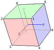
The faces that we wouldn't be able to see on a solid cube have the same property. For example, the face opposite the blue face is face 1 (vertices 5 8 7 6). At first glance it might look like the vertices are listed in clockwise order but you must remember that you must view the face from the outside of the object (not through the object). Looking at the same cube from the other side we see:
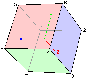
The pink face is face 1 and is parallel to the xy-plane at z = -1, the green face is face 3 and is parallel to the xz-plane at y = -1, and the blue face is face 6 and is parallel to the yz-plane at x = -1. Notice that for each of these faces, the vertices are listed in counter-clockwise order:
The requirement that the vertices of each face be listed in counter-clockwise order makes creating a polygon mesh data file significantly harder than creating the corresponding wireframe data file. Another problem with our polygon mesh model is that each edge is drawn twice since each edge is part of two different faces. Not only is each edge drawn twice, but it is drawn in opposite directions. For example, the edge from vertex 1 to 2 is part of face 2 where the edge is drawn from vertex 1 to vertex 2. This edge is also part of face four where it is drawn from vertex 2 to vertex 1. Unfortunately, drawing a line in one direction results in a slightly different set of pixels being used than the same line drawn in the other direction. As a result, drawing the same line in both directions often leads to lines with extra pixels.
At this point, you might be wondering why we would use a mesh model instead of a wireframe model. The answer is that using a mesh model makes it easy to draw only the faces that would be visible to the eye and not the faces on the back of the model that we wouldn't be able to see if the sphere were solid. The sphere on the left has had all of its faces drawn rendering it as a transparent object. The sphere on the right has had only its front faces drawn rendering it as a solid (opaque) object.
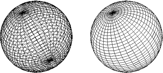
One technique used to remove the back faces from a rendered image is called back-face culling. Conceptually, as we go through the list of faces, we cull out (pick out and remove) the faces that are facing away from the viewer. This is, of course, only an analogy. In reality, we do not remove anything from the list; we simply ignore the back faces during the rendering process.
To see how the back-face culling process works we need to know a little bit about vectors. A vector is a directed line segment. The magnitude of a vector is the length of the line segment. For any face on a polygon mesh model we construct a vector from the first vertex to the second vertex and another vector from the second vertex to the third vertex. We are assuming that these two edges are not collinear (which is certainly reasonable). In the image below, we'll use face 2 from our cube as an example:
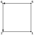
The first vector goes from the first vertex (vertex 5) to the second (vertex 6). The second vector goes from the second vertex to the third (vertex 2). Notice that first, second, and third refer to the order in which the vertices are listed for the face in the mesh model data file. To create a vector from one point to another you simply subtract the coordinates of the first point from the coordinates of the second point:
v1.dx = p6.x - p5.x = -1 -  1 = -2
v1.dy = p6.y - p5.y =  1 -  1 =  0
v1.dz = p6.z - p5.z = -1 - -1 =  0

v2.dx = p2.x - p6.x = -1 - -1 =  0
v2.dy = p2.y - p6.y =  1 -  1 =  0
v2.dz = p2.z - p6.z =  1 - -1 =  2
Notice that the first vector is parallel to the x-axis and points in the negative x direction. The second vector is parallel to the z-axis and points in the positive z direction. The cross product of these vectors is a vector that is perpendicular to the face and points outward. Here is how to calculate the cross product of two vectors (v3 = v1 x v2):
v3.dx = v1.dy * v2.dz - v1.dz * v2.dy =  0*2 -  0*0 = 0
v3.dy = v1.dz * v2.dx - v1.dx * v2.dz =  0*0 - -2*2 = 4
v3.dz = v1.dx * v2.dy - v1.dy * v2.dx = -2*0 -  0*0 = 0
Notice that the cross product is parallel to the y-axis (and thus perpendicular to face 2) and points in the positive y direction (outward):
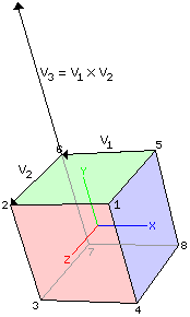
The cross product is said to be a surface normal (meaning that it is perpendicular to the surface or face). If the surface normal of a face points towards the viewer, the face should be rendered; otherwise the face should be ignored. In our case, the viewer is looking down the positive z-axis. Consequently, a surface normal will point towards the viewer if and only if its z-component is positive. Back-face culling is performed by calculating the surface normal for each face in the face list and drawing only the faces for which the z-component of the surface normal is positive.
For objects with closed convex surfaces, back-face culling is the only operation needed to generate a rendering that eliminates hidden faces. A closed surface basically means it doesn't have any holes in it (such as an open box). A convex surface basically means it doesn't have any indentations. A cube, an octahedron, and a sphere all have closed convex surfaces:

For an object whose surface is not closed and/or not convex, back-face culling is not enough. In the chess piece and vase images below, only front-faces have been rendered. However, some of those front-faces are behind closer front-faces. A more sophisticated algorithm is needed to detect when a front-face obscures another front-face that is farther away.
