Percents Lab
Objectives
- Learn how to enter numbers, text, and expressions in Excel.
- Learn how to format cells in Excel.
- Learn how to model markup, discount, and sales tax problems in Excel.
- Learn how to use Excel's Goal Seek tool.
Running Excel
Log-in to your user account and then double-click on the Excel icon
![]() .Depending on
how your computer is set up, you may find the Excel icon on the desktop, the
taskbar at the bottom of the screen, and/or the start programs menu.
.Depending on
how your computer is set up, you may find the Excel icon on the desktop, the
taskbar at the bottom of the screen, and/or the start programs menu.
Excel Worksheet
Conceptually, an Excel file is a workbook containing multiple worksheets. Each worksheet contains a rectangular grid of cells. A very small section of a worksheet is shown here:
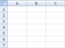
The rectangular grid of cells consists of vertical columns and horizontal rows. The first column is A, the second is B, the third column is C, and so on. After the first 26 columns, the columns are identified by 2-letter sequences (AA, AB, AC, ... AZ, BA, BB, BC, ... BZ, CA, ..., and so on). Once you go past column ZZ, the columns are identified by 3-letter sequences (AAA, AAB, AAC, etc). The very last column is identified as XFD. (If you are curious, there are 16,384 columns in an Excel worksheet.)
The rows are numbered from top to bottom starting with row one at the top. There are 1,048,576 rows. (That means there are a total of 17,179,869,184 cells in an Excel worksheet but, I assure you, we will never use more than a tiny fraction of them.)
Each cell is uniquely identified by its column and row identifiers. The column identifier always precedes the row identifier. Cell A1 is the cell in the upper-left-most corner. Cell XFD1 is the cell in the upper-right-most corner. Cell A1048576 is the cell in the lower-left-most corner, and cell XFD1048576 is the cell in the lower-right-most corner.
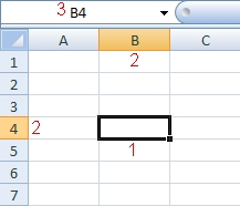
You can manipulate the contents of a cell only if it is active. The active cell is indicated three different ways as illustrated below.
- It is surrounded by a dark border.
- Its column and row identifiers are highlighted.
- Its address is displayed in the cell address box above the workbook on the far left of the screen.
You can move around the worksheet using the scroll keys or the mouse. If you want, you can also type a cell address in the cell address box and Excel will go directly to that cell.
Each cell on a worksheet can contain one of four things: nothing (it is empty), text, a number, or an expression. Cells containing text are often used as column headings or row headings.
Mathematical Model of Retail Price
A mathematical model usually has three basic components: output, input, and process. The output represents what it is we are trying to determine. In the simplest models this might be a single result often referred to as "the answer". The input represents data that we are given about the problem that we are modeling. The process refers to the steps that need to be taken in order to find the output based on the values of the input.
We will begin with a very simple problem. Given the wholesale price of an item and the markup rate, what is the retail price of the item? The output is the retail price since that is what we are trying to determine. The input is the wholesale price and the markup rate since both of these must be known in order to find the retail price. The process is the formula that we must implement to calculate the retail price:
Retail Price = Wholesale Price + Wholesale Price * Markup Rate
or
Retail Price = Wholesale Price * (1 + Markup Rate)
We will implement this simple model on an Excel worksheet. Read each numbered instruction all the way through before you do what it says.
Entering Text into a Cell
Cells containing text are often used as column headings or row headings. To enter text, go the cell in which you want to enter the text and then type in the text.
1. Click on cell A1.
2. Type in the text, "Wholesale Price". By common convention, the text that you are to enter is what appears between the quote symbols. Do not enter the quotes as part of the text.
3. Click on cell A2 and enter the text, "Markup Rate".
4. Enter the text, "Retail Price", in cell A3.
Entering a Number into a Cell
The process for entering a number into a cell is basically the same as for entering text. Move to the desired cell and type in the desired number.
1. Click on cell B1 and type in the number 299.99. Notice that, by common convention, a number is not enclosed in quotes.
2. Enter the number 0.25 in cell B2.
The text you entered in cell A1 identifies the value you just entered in cell B1. That is, the wholesale price is 299.99. Similarly, the markup rate is 0.25 (the decimal equivalent of 25%). Notice that cells B1 and B2 represent the input to this mathematical model.
Entering an Expression into a Cell
The output of this mathematical model is the retail price which will appear in cell B3. This is a calculated result. That is, we must process the input values in order to determine the output value for this model. Earlier, we identified two different (but algebraically equivalent) processes for calculating the retail price of this item. Let's begin with the first equation:
Retail Price = Wholesale Price + Wholesale Price * Markup Rate
1. Click on cell B3 and type "=B1+B1*B2". Since you are entering text rather than a number, you are to enter only what comes between the quotes. Excel interprets any text that begins with the equal sign as an arithmetic expression. Consequently, every expression you enter into Excel must begin with the equal sign. Otherwise, Excel will interpret your entry as ordinary text rather than an arithmetic expression.
The cell references in this expression tell Excel where to find the input values (i.e., B1 represents the wholesale price, and B2 represents the markup rate). Excel will retrieve these values, perform the indicated arithmetic operations and display the result (the retail price) in cell B3. You should have gotten a retail price of 374.9875.
Now lets implement the process using the second equation:
Retail Price = Wholesale Price * (1 + Markup Rate)
2. Click on cell B3 and type "=B1*(1+B2)". (It is not necessary to delete the previous entry first. When you click on a cell and start typing, anything already in the cell will be replaced by your new entry.) You should get the same value as before.
Both of these formulas illustrate a very important property of a good worksheet. Excel expressions should always use cell references whenever possible.
I want to show you another way to enter cell references in an Excel expression. As always, read each instruction all the way through before you do anything.
3. Click on cell B3 and type just the equal sign (and nothing else). This will clear the cell and begin the entry of a new Excel expression.
4. Click on cell B1 (which contains the wholesale price). When you click on a cell while entering an expression, Excel types the cell reference into the expression for you.
5. Type "*(1+".
6. Click on cell B2 and Excel will type in the cell reference for you.
7. Finish the expression by typing in the closing parenthesis and tap the Enter key.
What I want you to notice is that instead of typing in the cell references manually, you can click on the cell you want and let Excel type in the cell reference for you.
Formatting Cells
At this point, your Excel workbook probably looks something like this:
While the mathematical model has been correctly implemented, it doesn't look very nice. We can fix that by formatting the cells in our workbook. Formatting a cell does not change the contents of a cell; just its appearance. Excel applies default formats when you enter something into a cell. For example, when you entered the text in cells A1:A3 (A1 through A3), the text appeared to extend into the adjacent cells in column B. However, as you entered other content into cells B1:B3, that new content was displayed instead. As a result, the appearance of the labels in A1:A3 changed to a truncated version of the text. However, the text itself was not changed in any way.
The value displayed in cell B3 is another example of a default format. Even though you entered an expression into cell B3, Excel displays the result obtained by evaluating the expression rather than the expression itself. The cell appears to contain a number when, in fact, it contains an expression.
Adjusting the Width of Column A
First, let's adjust the width of column A so that we can see the row headings.
1. Using your mouse, point at the right edge of column A (i.e., between column A and B) as shown below. Holding the left mouse button down, drag the mouse to the right until column A is wide enough to see all of the row headings. If you make it too wide, repeat the process except drag the mouse a little to the left to make the column narrower.
Formatting Dollar Amounts
The wholesale price and the retail price are dollar amounts and should be formatted accordingly. There are three commonly used formats for dollar amounts: currency, accounting, and comma. In the table below I entered the same numbers in both columns; 1234.567 in the left column and -1234.567 in the right column:
Excel's general format (the default format) basically displays just what you type in.
Excel's currency format displays a dollar sign immediately to the left of the left-most digit, adds a comma separator (when needed) and displays the value to the nearest penny. Negative values are indicated by adding a minus sign to the left of the dollar sign. You can modify the currency format to omit the dollar sign if desired.
The accounting format displays a dollar sign all the way to the left in the cell containing the number, adds a comma separator (when needed) and displays the value to the nearest penny. Negative values are displayed by enclosing the number in parentheses. I haven't shown it here, but a value of zero is displayed as a hyphen rather than the numeral zero (0).
The comma format is the accounting format without the dollar sign.
It doesn't really matter which format you use as long as you are consistent. In this lab exercise, we will be using the currency format.
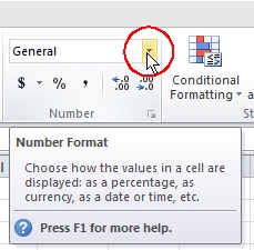
2. Click on cell B1 and then open the format menu in the number format section of the home toolbar:
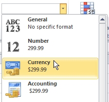
3. In the format menu, select the currency format:
4. Repeat this process for the retail price in cell B3.
Formatting Percent
5. Click on cell B2 and then click on the percent format button:
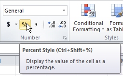
You could also have opened the format menu as you did above and then chosen the percentage format from the menu. A third approach would be to use the keystroke combination indicated in the graphic above. I think the easiest approach, however, is to use the percent format button as we did.
In case you are wondering, the button with the dollar sign is a shortcut for applying the accounting format and the button with the comma is a shortcut for applying the comma format.
Adjusting the Width of Column B
Let me show you another way to adjust the width of a column.
6. Point to the right edge of column B (between columns B and C). Instead of dragging the mouse to adjust the width of column B, double-click the left mouse button. Excel will automatically adjust the width of column B based on the values currently displayed in the column.
With these formatting changes, your worksheet should look like this:
What-If Analysis
One of the main advantages of implementing a mathematical model in Excel is that it becomes very easy to perform what-if analysis. For example, what if the wholesale price were changed to 149.99 and/or the markup rate was changed to 35%? Anytime we change an input value, Excel will automatically recalculate the expressions that generate the output values.
1. Click on cell B1 and enter 149.99. Notice that Excel recalculates the expression in cell B3 and displays the retail price as $187.49
2. Click on cell B2 and enter 35. Again, Excel recalculates the expression in cell B3 and displays the new retail price as $202.49. In a previous step,we told Excel that the value in cell B2 represents a percentage. As a result, when we entered 35, Excel interpreted that as 35% rather then the decimal value 35 which would have been 3,500%.
Excel also provides a very powerful tool for performing what-if analysis that would normally require constructing a new model. For example, what if the wholesale price was $330 and the retail price was $450. What is the markup rate?
One way to answer that question would be to solve the retail price expression for the markup rate. That would give us a new model in which wholesale price and retail price are the inputs and markup rate is the output. With Excel, however, we can find the markup rate using our original model. We don't need to create a new one.
3. Set the wholesale price in B1 to $330.
4. Click on cell B3.
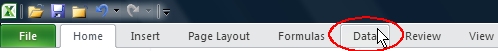
5. Open the Data toolbar:
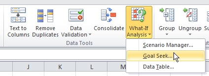
6. In the What-If Analysis menu, select the Goal Seek option:
7. Because we had already clicked on cell B3, that cell already appears in the Set Cell edit box of the Goal Seek dialog window. We want to set the value of B3 to 450 by changing the value in cell B2:
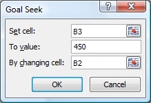
8. When you click the OK button, the markup rate will change to 36%. You need to click another OK button to return to your worksheet.
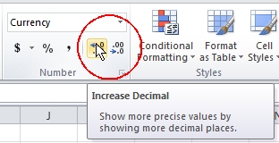
9. You can use the Increase Decimal and Decrease Decimal tool buttons back on the Home menu to change the number of decimal places displayed in a cell. Click on cell B2 and then click the Increase Decimal button a couple of times to display the markup rate to two decimal places (36.36%).
10. Save your workbook as "PercentLab" using the Save option on the File menu. It doesn't make any difference where you save the file as long as you do not save it on the hard drive of one of the computers in a computer lab. That is not permitted and if you do so, the file will be erased and you will not be able to recover it. I suggest you save your file in your user space.
Mathematical Model of Sale Price
Create a mathematical model that calculates the sale price of an item given its retail price and the discount rate. We'll use the same worksheet that we used for the retail price model.
1. Enter the row headings in cells A6:A8:
2. Enter the expression for the sale price in cell B8. Remember that this expression will use a reference to cell B6 (retail price) and cell B7 (discount rate). It is not necessary to enter a number in either cell before entering the expression for the sale price. Excel interprets an empty cell as zero. Consequently, you should get a value of zero in cell B8 when you enter your expression.
3. Enter a retail price of 84.99. The sale price should also change to 84.99 because cell B7 (the discount rate) is empty and interpreted as a 0% discount (no discount).
4. Enter a discount rate of 10%. You can do this two different ways. If you type in "10%" then Excel will automatically format the cell using the percentage format. If you enter the decimal equivalent of 0.10 then you will have to manually format the cell to display using the percentage format. The sale price should change to 76.491.
5. Format the retail price and sale price cells using the currency format. Your worksheet should look like this:
6. Change the retail price in cell B6 to 119.49. The sale price should change to 107.54.
7. Change the discount rate to 15%. The sale price should change to 101.57.
8. Find the original retail price if the sale price is 199.99 and the discount rate is 20%. Begin by setting the discount rate in B7 to 20%. Then click on cell B8 (the sale price). Finally, use the Goal Seek tool to set the value of cell B8 (the sale price) to 199.99 by changing cell B6 (the retail price). You should find that the retail price was $249.99.
Mathematical Model of Final Price
Create a mathematical model that calculates the final price of an item given its sale price and the sales tax rate. We'll use the same worksheet that we used for our other two models.
1. Set up your model in cells A11:B13 (the rectangular block of cells from A11 at the upper left to B13 at the lower right). Use your other two models as a guide. Don't forget that building the model includes properly formatting the cells.
2. What is the final price if the sale price is 199.99 and the sales tax rate is 6%? (You should get $211.99.)
3. What if the tax rate were 4.5% instead of 6%? (You should get a final price of 208.99.)
4. What if the sale price was 149.49 and the final price was 154.97. What is the sales tax rate displayed to 2 decimal places? (You should get 3.67%.)
Putting it All Together
Create a mathematical model whose output is the final price given the wholesale price, the markup rate, the discount rate, and the sales tax rate.
1. Set the model up in cells D1:E5 as illustrated below. Cells E1:E4 will contain input values. Cell E5 will contain the expression that calculates the final price.
2. Enter an expression in cell E5 that will calculate the final price based on the values in cells E1:E4. You should make every effort to figure out the expression on your own. If you don't know where to start here is a link to a hint. If you are still stuck, then follow this link to get some help.
3. Set the wholesale price to $400, the markup rate to 20%, the discount rate to 20%, and the sales tax rate to 5.5%. What is the final price to the customer? Your model should look like this:
4. Suppose the wholesale price, the markup, and the sales tax rate stay the same. What was the discount rate (to two decimal places) if the final price was $455.76? Using the goal seek tool to set the value in cell E5 to 455.76 by changing cell E3 (the discount rate), you should get a discount rate of 10.00%
5. Save your workbook and let me look at it.
6. Log off the computer. If you forget to log off, the next person to use the computer will have access to your email and all of the files stored in your user space. A malicious person could delete all of your email and all of your files and even try to access inappropriate web sites using your credentials. Always log off before you leave.
My Worksheet
If you are unclear about something or just want to see my workbook, here is a link to it: PercentLab.xlsx