

In this course, we will find left-tail probabilities by looking them up in a table or using Excel's NORMDIST function. However, one might well wonder how the table values were calculated and how Excel's NORMDIST function works. This page contains a brief description of how left-tail probabilities are calculated.
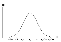
The graph of a normal distribution with a mean of μ and a standard deviation of σ is shown below. Beside the graph, is the corresponding mathematical function.

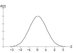
For the standard normal distribution, μ = 0 and σ = 1. The graph and corresponding function are shown here:
![]()
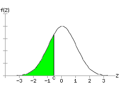
For any normal distribution, the left-tail probability is the area under the curve to the left of some specific value divided by the total area under the curve. For the standard normal distribution, the total area under the curve is exactly 1. Consequently, the left-tail probability, P(z < c), is just the area under the curve and to the left of c. This area is the integral of the standard normal distribution function from negative infinity to c:

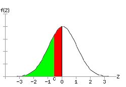
Given the symmetry of a normal curve, the left-tail area can also be calculated as 1/2 minus the area from c to 0. In the picture below, the green area is 1/2 minus the red area.

In general the integral from a to b is the negative of the integral from b to a. In our case we can write:

Making this substitution we get:

Bringing the constant out in front of the integration sign, we obtain:

The only problem, and it's a biggie, is that the integral in this formula cannot be found.
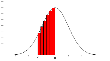
Since we cannot find the left-tail area by integration, we must resort to other techniques that allow us calculate accurate approximations of the desired area. One approach is to divide the base of the area into subintervals and for each subinterval, approximate the area under the curve using a rectangle. In the image below, the sum of the areas of the rectangles is approximately equal to the area under the curve from c to 0. Notice that each rectangle includes a little bit of area above the curve but misses a little bit under curve. These tend to balance out giving a good approximation. In general, the greater the number of subintervals, the better the approximation.
There are numerical methods that allow us to estimate the area under the curve using simple arithmetic. Here is the formula for the area under the curve where I've emphasized that the limits of integration correspond to specific values of z:

Making the substitution
![]()
in the integral yields this result:

For a moment, consider just the
integral in this formula. The Taylor series representation of the
function, ![]() ,
is given by:
,
is given by:

Substituting the Taylor series for the exponential function in the integral and using the fact that the integral of a sum is the sum of the integrals, we obtain the following:
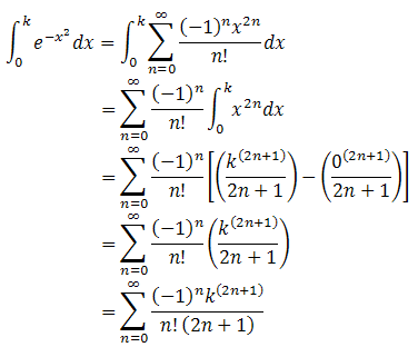
Substituting this result into our formula for the left-tail area yields:

The Excel workbook LeftTailCalculation.xlsx compares the results obtained using Excel's NORMDIST function and the results obtained by using the first 21 terms of the infinite sum shown here. To four decimal places, the values generated by the two methods are exactly the same. Better results can be obtained by simply using more terms of the sum.
Modern computer software and scientific calculators use this same basic approach to calculate left-tail areas. However, they use a much more computationally efficient version of the formula shown here. Before there were calculators and computers, the left-tail areas were calculated by hand (paper and pencil) using these same techniques. Can you imagine how tedious that must have been?