
One of the most fundamental sets of descriptive statistics is the five-number summary: minimum, first quartile, median (second quartile), third quartile, maximum. It is a useful summary regardless of the shape of the distribution of data values (unlike the mean and standard deviation which are most appropriate with distributions that are normal or nearly so).
The procedure for finding the five-number summary is covered early in any introductory statistics book. Yet, it is interesting to note that such an elementary and fundamental topic is almost always accompanied by a caveat as illustrated by this quote from a popular textbook:
"Some software packages use a slightly different rule to find the quartiles, so computer results may be a bit different from your own work. Don't worry about this. The differences will always be too small to be important."
As a matter of fact, such a caveat is actually an understatement. Among the most commonly used statistics software packages, three different values may be generated for both the first and the third quartiles.
Conceptually, the three quartiles (Q1, Q2, and Q3) divide the list of sorted data into four categories:
and
For sample data, the location of the quartiles are interpreted as distances. The first quartile is at a position 1/4 of the way into the list, the second quartile is at a position 1/2 of the way into the list, and the third quartile is at a position 3/4 of the way into the list:
![]()
Sandy Koufax pitched for the Dodgers from 1955 to 1966 (the Dodgers moved from Brooklyn to Los Angeles in 1958). The numbers of games he won per year during his career are given below; sorted in ascending order.
![]()
To measure the distance to the location of the quartiles, you will need a special ruler:

Both the data set and the ruler are GIF graphics. You can print out both, cut out the ruler, and use it to measure distances into the list. (This hands-on exercise isn't absolutely necessary, but I think it will help you understand the issues involved.)
Depending on how you measured your distances (and assuming no arithmetic errors) you probably came up with one of the following values: 5.75, 6.5, or 7.25. Each of these results is generated by at least one commonly used software package.
You should have come up with a value of 12.5. Every software package yields the same result for the median.
You probably came up with one of the following values: 20.5, 22, or 23.5.
The algorithms for calculating the quartiles differ only in how the length of the list is measured.
This algorithm is used by Microsoft's Excel spreadsheet software. The length is measured as the distance between the first value and the last value in the list. A list with n elements has a length of n-1 and the quartiles are located at distances of 1/4(n-1), 1/2(n-1), and 3/4(n-1).
For our example data, the length of the list is 11:

The location of each quartile and its value are given in the table below.
| Q1 | Q2 | Q3 | |
|---|---|---|---|
| Location | 1/4(11) = 2.75 | 1/2(11) = 5.5 | 3/4(11) = 8.25 |
| Value | 7.25 | 12.5 | 20.5 |
This algorithm uses an intuitive measurement technique; one that would be used to measure a physical object. Excel also has a Q0 (the minimum) located at 0/4(n-1) which is location 0; the first value in the list. Q4 (the maximum) is at location 4/4(n-1) which is location n-1; the last value in the list.
The second algorithm is used by both the TI-83 calculator and the hand-calculation method but only when the number of values in the list is even. The length is measured from a point one half unit before the first value in the list to a point one half unit beyond the last value in the list. A list with n elements has a length of n and the quartiles are located at distances of 1/4(n), 1/2(n), and 3/4(n).
For our example data, the length of the list is 12:

The location of each quartile and its value is given in the table below.
| Q1 | Q2 | Q3 | |
|---|---|---|---|
| Location | 1/4(12) = 3.0 | 1/2(12) = 6.0 | 3/4(12) = 9.0 |
| Value | 6.5 | 12.5 | 22.0 |
This algorithm leads to an intuitive result for the length of the list. I suspect that most people, if asked "How long is a list of 12 values?", would say, "12". I suspect the way in which the length is measured is not as intuitive.
Minitab, SPSS, TI-83 (n odd) and the hand-calculation method (n odd) all measure the length from one full unit before the first value to one full unit after the last value. A list with n values has a length of n+1 and the quartiles are located at distances of 1/4(n+1), 1/2(n+1), and 3/4(n+1).
For our sample data, the length of the list is 13:

The location of each quartile and its value is given in the table below.
| Q1 | Q2 | Q3 | |
|---|---|---|---|
| Location | 1/4(13) = 3.25 | 1/2(13) = 6.5 | 3/4(13) = 9.75 |
| Value | 5.75 | 12.5 | 23.5 |
For this algorithm, both the measurement technique and the resulting length are, in my opinion, counter-intuitive.
Boxplots (sometimes referred to as box and whisker plots) are used to illustrate the five-number summary. A line (whisker) extends from the minimum value to the first quartile. A box extends from the first quartile to the third quartile with a vertical line indicating the median. A second line extends from the third quartile to the maximum. The interval between the first and third quartiles (the box) determines the interquartile range.
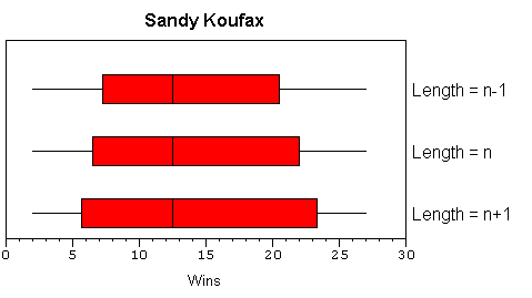
While the differences among the first and third quartiles we got above may "be too small to be important", they do lead to boxplots with different visual impressions. The width of the interquartile range and the length of the whiskers are noticeably different:

The table below summarizes the algorithms used by several common software packages and the hand-calculation method. Note that the TI-83 calculator implements the hand-calculation method. I'm sure the folks at Texas Instruments did this intentionally so calculator-generated results would agree with results generated by hand. However, it is also worth noting that this algorithm is inconsistent; calculating length one way when n is even and another way when n is odd.
| Length = n-1 | Length = n | Length = n+1 |
|---|---|---|
| Excel | TI-83 (n even) Hand-Calculation (n even) |
TI-83 (n odd) Hand-Calculation (n odd) Minitab SPSS |
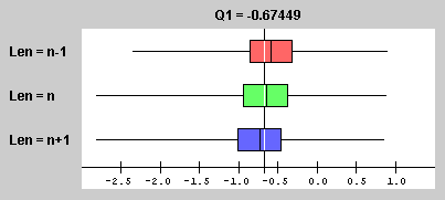
Fifty thousand simple random samples of size 10 were drawn from the standard normal distribution (μ=0 and σ =1). For each sample, the first quartile was calculated using each of the three basic algorithms. The boxplots for the distributions of sample first quartiles are shown here:

The vertical line near the center of the chart represents the first
quartile of the population
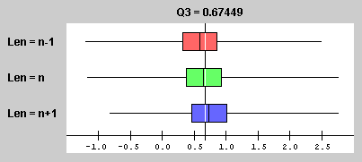
Here are the boxplots for the distributions of the third quartiles for this same experiment:

The vertical line near the center of the chart represents the third
quartile of the population
As the sample size increases, the differences among the results generated by the different algorithms diminish.
If you browser is capable of running Java Applets, you can run this experiment yourself with different sample sizes and different populations. Just run the Quartile Calculation Applet.
While implementing a quartile algorithm in software requires the ability to write a computer program, the underlying issues can be understood even by those who lack this skill. The first issue involves the way in which lists of data are stored as one-dimensional arrays in a computer. The second issue involves the mapping of the location of a quartile (measured as a distance) to the corresponding position with the one-dimensional array.
In a computer, a list of data is stored as a one-dimensional array. Each element in such an array is identified by its position (index) within the array. Historically, some languages (such as FORTRAN and BASIC) assign an index of 1 to the first value in an array and other languages (such as C, C++, and Java) assign an index of 0 to the first value. (Array processing is slightly more efficient if the index of the first element is 0.)
When implementing the quartile calculation algorithms, the location of a quartile (as a distance) must be converted to the corresponding index in the array. If the resulting index is not an integer, interpolation is used to calculate the value of the quartile.
Converting the location of a quartile within the list (as a distance) to the corresponding index turns out to be quite simple. In every case, the index is the location plus or minus a constant offset. The value of the offset is determined by two things: the algorithm used to determine the length and whether the first element in the array is assigned an index of 0 or an index of 1.
If the length of the list is measured as n-1, the location of the quartile and the corresponding index are exactly the same; the offset is zero. In the illustration below, the bold red numbers represent the indices of the corresponding data values.

If the length of the list is measured as n, the index is equal to the location minus one-half. In the example below, Q1 is at distance 3.0 which corresponds to an index of 2.5 (the value of Q1 is half-way between the values at indices 2 and 3).

If the length of the list is measured as n+1, the index is equal to the location minus one. In the example below, the first quartile is at distance 3.25 which corresponds to an index of 2.25 (the value of Q1 is one-fourth of the way between the values at indices 2 and 3).

If the length of the list is measured as n-1 then the index is equal to the location plus one. In the example below, the first quartile is at distance 2.75 which corresponds to an index of 3.75 (the value of Q1 is three-fourths of the way between the values at indices 3 and 4).

If the length of the list is measured as n then the index is equal to the location plus one-half. In the example below, the first quartile is at distance 3.0 which corresponds to an index of 3.5 (the value of Q1 is one-half of the way between the values at indices 3 and 4).

If the length of the list is measured as n+1, the location of a value and the corresponding index are exactly the same.

The table below summarizes the mappings between location (as distance) and the corresponding index for the three quartile calculation algorithms and the two types of arrays.
| Algorithm | Base 0 Array | Base 1 Array |
|---|---|---|
| Length = n-1 | Index = Location | Index = Location + 1.0 |
| Length = n | Index = Location - 0.5 | Index = Location + 0.5 |
| Length = n+1 | Index = Location - 1.0 | Index = Location |
I wouldn't be at all surprised to discover that the length = n-1 algorithm has its roots in a language that uses base 0 arrays and that the length = n+1 algorithm has its roots in one that uses base 1 arrays. In either case, the location and the index would be the same.