
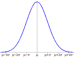
When something happens most of the time, we call it usual, or typical, or normal, or common. Most of the time, the population attribute being studied has a characteristic distribution of values. Because it is so common, this distribution is called the normal distribution. All normal distributions have several common properties (as illustrated in the graph below):
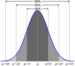
In addition, the proportion of measurements between given boundaries is the same for all normal distributions. For example, approximately 68% of the population will lie within one standard deviation of the mean, about 95% will lie within two standard deviations of the mean, and roughly 99% of the population will lie within three standard deviations of the mean:
Typically, only large populations are described as normally distributed because only large data sets will result in a smooth , symmetric distribution:

The distribution of sample values (taken from a normally distributed population) only approximate the bell-shaped curve of a normal distribution:

The standard normal distribution (illustrated in the graph below) is a normal distribution with a mean of 0 and a standard deviation of 1.
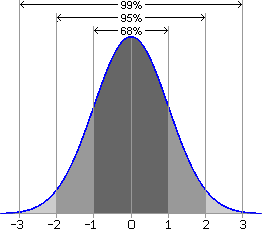
A value in any normal distribution can be converted to a standard score (also called a "z score"). For any given value "x", the standard score is found by dividing the corresponding deviation from the mean by the standard deviation. A standard score can be interpreted as the number of standard deviations to the left or the right of the mean.
![]()
Suppose the average height of all adult males is 69.72 inches with a standard deviation of 1.79 inches. To find the standard score corresponding to a height of 67 inches, find the deviation (67 - 69.72) and divide by the standard deviation (1.79):
![]()
A height of 67 inches, is 1.52 standard deviations to the left of (graphically) or below (numerically) the mean.
The ability to convert scores in a normal distribution to standard scores has a very practical application. Values from two different distributions can be compared by converting both to standard scores. Suppose, for example, that ACT scores are normally distributed with a mean of 24 and a standard deviation of 3.5 and that SAT scores are normally distributed with a mean of 550 and a standard deviation of 80. (These values are for illustrative purposes only; they are not accurate.)
Jack had an ACT score of 30 and Jill had an SAT score of 690. Which student had the better score? The answer can be determined by converting both scores to standard scores and comparing them.
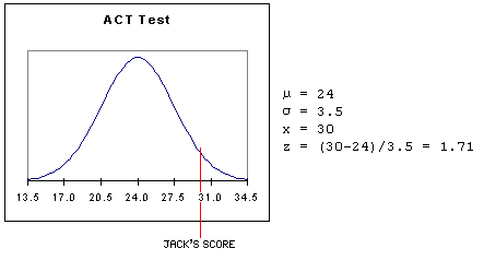
Jack's ACT score was 1.71 standard deviations above the mean ACT score.
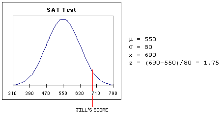
Jill's SAT score was 1.75 standard deviations above the mean SAT score. Comparing the standard scores, Jill's score of 1.75 is slightly better than Jack's score of 1.71.
One of the most important properties of the standard normal distribution is that the total area under the curve is exactly one. Consequently, areas under the curve can be interpreted as probabilities. Left-tail probability tables are used to look up the area to the left of a given score (see illustration below). For a given standard score c, the left-tail area corresponds to the probability P(z < c). This area can also be interpreted as P(z <= c) since the inclusion of the equals sign does not change the probability. This is true for all probabilities based on the standard normal distribution. (For those who have taken some calculus, the left-tail calculation page provides a description of how these left-tail probabilities are actually calculated.)
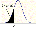
The link in this paragraph will take you to a left-tail probability table. The instructions for using the table appear below the table. This was done so that if you print the table, as much of it as possible will be on one page. Left-tail Probability Table.
There are three basic kinds of probability problems that can be solved using these tables:
Remember that any of the inequalities can be replaced with the corresponding "or equal to" with no change in the result. In all three kinds of problems there are two basic steps:
These are the easiest problems to solve since the answer comes directly from the table. The entry in the table for a given value c is P(z < c).
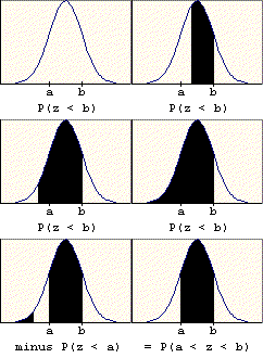
A problem of this type asks for the probability that a value chosen at random is between two given values (a and b). The probability is found by subtracting the table entry for "a" (the smaller value) from the table entry for "b" (the larger value). The graphic below illustrates the basis for this procedure.
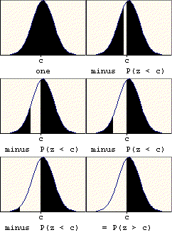
A problem of this type asks for the probability that a value chosen at random will exceed a given value (c). The probability is found by subtracting the table entry for "c" from one. It is based on the following property of probability: P(E) = 1 - P(E'). The probability of success is one minus the probability of failure. The right-tail area (success) is one minus the left-tail area (failure). The graphic below illustrates this property.
