
Excel's COUNTIF function counts the number of values in a specified range of cells that satisfy a given condition. The COUNTIF function has two arguments: the specified range of cells and the condition that must be met:
=COUNTIF(range, condition)
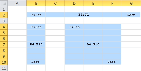
The range is specified by two cell references separated by a colon. This is the same notation that we have been using in the lab instructions to refer to a block of cells. The two cell references refer to the first and last cells within a single row of cells, the first and last cell references within a single column of cells, or the first (upper-left) and last (lower-right) cells in a rectangular block of cells. Here are some examples:
The condition or criterion specifies what property the value in a cell must have in order to be counted. In this course, the condition will always involve a relationship and a value and will be written in this format:
Relationship & Value
The relationship is always in quotes and can be any of the following: "<", "<=", ">", ">=", or "=". The value can be a number, a cell reference, or an Excel expression. Here are some examples:
"="&C5 means a cell will be counted if its value is the same as the value in C5.
"<"&(C5+2) means a cell will be counted if its value is less than the value of C5 plus 2.
">="&(F4-3) means a cell will be counted if its value is greater than or equal to the value of F4 minus 3.
The COUNTIF function counts all of the cells in the specified range that satisfy the specified condition. Here are some examples:
=COUNTIF(B2:G2,"="&H3) means count the number of cells in the range B2 through G2 that have a value equal to the value in cell H3.
=COUNTIF(D4:F10,"<"&(A13+5)) means count the number of cells in the range D4 through F10 that have a value less than 5 plus the value in cell A13.
=COUNTIF(B4:B10,">="&(D13-2)) means count the number of cells in the range B4 through B10 that have a value greater than or equal to the value in cell D13 minus 2.
Suppose that you are a member of a consumer advocacy group investigating the Mars Candy Company and specifically the number of M&Ms that come in a package.
1. I have not provided a worksheet for this lab. Instead, you will start with a blank workbook. Double-click on the "Sheet 1" tab and change the tab text to "M&Ms".
2. Enter your name in cell A1.
3. Set up column headings exactly as shown below:
4. Save your workbook as "StatLab1".
A random sample of 29 packages of M&Ms was collected and the number of M&Ms in each package counted. Here are the results.
58, 60, 57, 56, 55, 58, 60, 59, 56, 56, 55, 58, 57, 55, 55, 56, 56, 56, 54, 57, 57, 57, 59, 57, 52, 54, 54, 58, 58
1. Enter this data, in the order listed, into the "Raw Data" column of your worksheet. (Column C, the "# of M&Ms" column, will be used later as part of the ungrouped frequency distribution.)
2. Save your workbook.
1. Go through the list of raw data values to find the smallest and largest values in the list. Enter the smallest number in the first cell of the column labeled "# of M&Ms". Fill the remainder of the this column with successively higher values up to and including the largest value in the list.
2. In cell D4, use the COUNTIF function to count the number of packages that contained the smallest number of M&Ms. You will be copying this formula down the column so be careful to use absolute references where needed. When you copy this formula down the column, the range of cells containing the raw data is always the same but the cell containing the specific value that you are counting changes. Verify that you get the correct value before continuing. Make every effort to figure out the correct expression on your own. Help.
3. Use the fill handle to copy the COUNTIF formula down the rest of the column.
4. The sum of the frequencies should always add up to the number of values in the data set. Click on the blank cell immediately below the last value in your "Frequency" column and click the auto sum tool:
![]()
When you click the AutoSum tool button, Excel will generate a formula that gives the sum of the values in the column above. This sum should equal the number of values in the data set (i.e., the sample size, n).
5. Save your workbook.
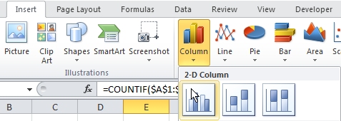
You've created many line charts in previous lab projects. Creating a column chart is very similar. There are really only two differences. When you go to insert a new chart, you must choose a column chart rather than a line chart:
The second difference is that for a column chart you want the vertical axis to cross between tick marks. This is the default, so you will not need to change the setting as you did for line charts.
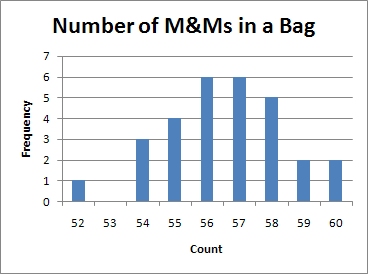
Prepare a column chart illustrating the frequency distribution. Your chart should look like this:
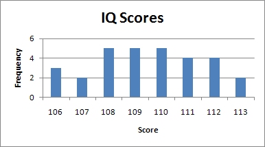
The numbers below represent IQ scores for a random sample of 30 students.
109, 106, 106, 110, 108, 110, 108, 106, 110, 108, 110, 112, 110, 109, 109, 112, 107, 113, 108, 107, 113, 109, 111, 111, 111, 108, 109, 112, 112, 111
1. Go to the second worksheet (Sheet2). Rename this sheet, "IQ Scores". Enter your name in cell A1.
2. Set up your worksheet as shown here:
3. Enter the data given above into column A starting in cell A4.
4. Prepare a frequency distribution and summarize the data with a column chart. Your column chart should look like this:
5. Save your workbook.
The data below lists the number of absences for each student in a class.
0, 2, 0, 1, 0, 0, 2, 0, 0, 0, 0, 2, 4, 4, 5, 1, 0, 2, 0, 0, 2, 2, 0
Set up a worksheet named "Absences" to generate a frequency distribution and a column chart that illustrates that distribution.
A titration experiment in a chemistry class resulted in the data (in milliliters) below.
0.109, 0.111, 0.110, 0.110, 0.105, 0.110, 0.111, 0.110, 0.110, 0.111, 0.109, 0.111, 0.109, 0.112, 0.109, 0.109, 0.111, 0.110, 0.112, 0.112, 0.109, 0.110, 0.110, 0.109, 0.113, 0.108, 0.105, 0.110, 0.109, 0.109, 0.110, 0.110, 0.110, 0.104, 0.109, 0.110, 0.111
Insert a new worksheet named "Titration" into your workbook and generate an ungrouped frequency distribution and a column chart that illustrates that distribution.
Some MAT 120 students were asked to record their age (in years) with the following results: 18, 18, 19, 19, 22, 20, 18, 22, 18, 20, 20, 18, 18, 18, 18, 19, 21, 18, 18, 18, 20, 18, 23, 19, 18, 18, 18, 18. Insert a new worksheet named "Ages" and generate an ungrouped frequency distribution based on this data. Illustrate your distribution with a chart.
You can check your work by looking at FreqDist01Done.xlsx.