In Excel, you can use the Increase Decimal (or Decrease Decimal) tool buttons to control the display of cell values:
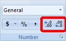
However, the actual value is unchanged. Changing the display format of a value does not change the value itself. In finance, the calculated values must actually be rounded off to the nearest cent not merely displayed to the nearest cent. To do this, you will need to use Excel's ROUND function.
=ROUND(expression, decimal places)
The expression argument is usually a formula that generates the value that is to be rounded off. The second argument, decimal places, specifies the number of decimal places to which the value generated by the expression will be rounded.
![]() Follow
these instructions carefully to make sure that your Excel file is saved in the
correct folder in your user space. I suggest you read all 6 steps before you do
anything.
Follow
these instructions carefully to make sure that your Excel file is saved in the
correct folder in your user space. I suggest you read all 6 steps before you do
anything.
1. Run
![]() . (In
general, Mozilla Firefox seems to exhibit less weird behavior than Microsoft
Internet Explorer.)
. (In
general, Mozilla Firefox seems to exhibit less weird behavior than Microsoft
Internet Explorer.)
2. Right-click (click the right mouse button) on the link to the Excel file: Lab01.xlsx.
3. In the pop-up menu, select the Save Link As... option:
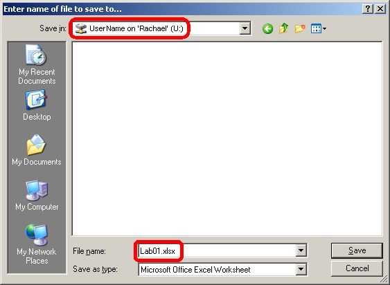
4. In the file save dialog box, navigate to your user space in the Save in section at the top. Of course, you will use your own user name and the server name will probably be different, but the graphic below illustrates the basic idea:
5. Click the Save button in the lower right corner.
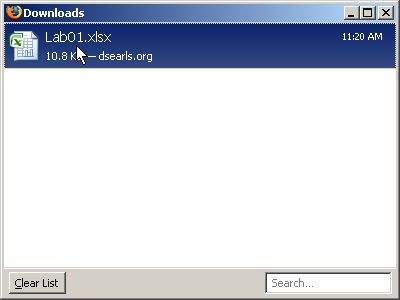
6. To open the downloaded file in Excel, double-click the file name in the Downloads dialog:
If you prefer, you can also run Excel and open the downloaded file from within Excel.
1. $1,000 is invested for five years in a savings account paying 4% compounded monthly. In the steps that follow, you will be performing these tasks:
2. Activate the "Compound Interest" sheet and enter your name in cell B1.
3. Calculate the periodic rate and number of periods:
a. The periodic rate is found by dividing the nominal rate (r) by the number of periods per year (ppy). Using cell addresses for both the nominal rate and the number of periods per year, enter the formula for periodic rate in cell B5. Help
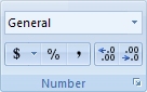
Format the periodic rate as percent to three decimal places using the tools in the number group.
b. The number of periods is found by multiplying the time in years (t) by the number of periods per year. Using cell addresses for both the years and the number of periods per year, enter the formula for the number of periods in cell B7. Help
4. Calculate future value and total interest using formulas:
a. In cell B9, calculate the future value using the compound interest formula A=P(1+i)n. Display the result using the currency format (the tool button with the dollar sign on it) to two decimal places. Help
b. In cell B10, enter the interest earned formula (I=A-P) using cell references to replace the variables. Display the result using the currency format.
c. Highlight the cells containing the future value and the interest earned (B9:B10). Set the background color to light gray. Add borders around the cells and set the font to bold. This will allow you to distinguish between your initial data and your calculated results.
5. Create a table showing the initial balance, interest earned, and new balance at the end of each period:
a. Highlight the first two cells under the heading "End of Period" (these cells contain the values 0 and 1). Drag the fill handle (the little black square at the lower right) until you have highlighted as many rows as there are periods (60 in this particular problem). Since you highlighted two cells containing consecutive integers, Excel will continue the sequence. As you drag the fill handle down, Excel will show you what the final value in the sequence will be. Keep dragging until you reach the desired value and then let the mouse go.
b. Period zero is a fictitious period that is included to make graphs look nicer. The final balance at the end of period zero is the amount of money deposited into the account. In cell D13, enter a formula containing a cell reference to the present value. Remember, always use cell references in formulas whenever possible. Help
c. The initial balance for each period (starting with period 1) is the final balance from the previous period. In cell B14 enter a formula containing the correct cell reference for the new balance at the end of period zero. Help
d. The periodic interest is the amount of interest earned during the period. In every financial table we do in this course, the periodic interest is the value of the investment at the beginning of the period multiplied by the periodic interest rate. In cell C14, the correct formula is:
=B14*B5However, there is a problem. If we copy this formula down one row it will become =B15*B6. Try it! Do you see the problem? In row 15, the initial balance is, indeed, stored in cell B15 so that is correct. However, the periodic rate is not stored in B6; it is still up in cell B5.
When you copy a formula, Excel normally alters the cell reference accordingly. When you copy a formula down a column, the row references are automatically adjusted and when you copy a formula across a row, the column references are automatically adjusted. In most cases, this is what you want. For example, as we copy the periodic interest formula down the column, we want the reference to the initial balance to change accordingly.
Occasionally, however, we want to copy a formula without automatically adjusting a cell reference. In this case, we want the reference to cell B5 to remain unchanged as we copy the formula down the column because the periodic rate is always in cell B5 whether we are in row 14 or row 24 or any other row. To tell Excel that we do not want it to adjust a cell reference (row or column), we place a $ in front of the reference. Here is the modified formula:
=B14*B$5It is not necessary to put a $ in front of the B (making it $B$5) because the column address will not change anyway if all we do is copy the formula down.
A cell reference (row or column) preceded by a $ is called an absolute reference because it will not change when the formula containing the reference is copied. A cell reference without the $ is called a relative reference because it is subject to change when the formula containing the reference is copied. By default, cell references in Excel are relative. You have to add the $ to make them absolute.
If you haven't already, enter the correct formula for the periodic interest in cell C14.
e. Modify cell C14 to use the ROUND function to round the periodic interest to the nearest penny. You should always round the periodic interest to the nearest penny. Help
f. The new balance is the initial balance plus the periodic interest. Enter the appropriate formula in cell D14. Help
g.
Copy the formulas in cells B14 through D14 (B14:D14) down one row. (Highlight the three cells and drag the fill handle down one row.) Make sure that all the values are correct. If they are not, make any corrections in the formulas in row 14 and try again. When the values in row 15 are correct, drag the fill handle down the rest of the table (or double-click the fill handle). The final balance after 60 periods should be $1,221.00 confirming the result you got earlier using the future value formula.
h Highlight the cells in the periodic interest column. At the very bottom of the worksheet, Excel will list the average interest per period(3.68), the count (60) and the sum (221.00). Notice, in particular, that the sum is the same value you got using the total interest formula in cell B10. In general, the value given by the formula should be thought of as only a good approximation since it doesn't take rounding into account. The sum of the interest payments in the table will always be the correct value.
i. If necessary, highlight the body of your table (excluding the first column which lists the periods) and click the comma format button in the number group.
6. Save your workbook.
7. Follow the steps below to create a line chart illustrating the growth of the balance in the savings account.
a) Insert the Chart
When creating a chart illustrating the growth (or, later on, the decline) of the balance in an account, always use the final or new balance column. Highlight the column containing the new balance values. Click the Insert tab:
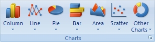
In the Charts group, select the type of chart you want to create:
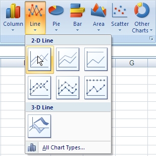
Once you have selected a chart type, select the desired subtype. In the illustration below, the user selected the line chart button and then choose the subtype that displays only two-dimensional lines (without data markers):
b) Set the Horizontal Axis Labels
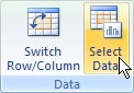
Use the values in the end of period column as the horizontal axis labels. Click on the Select Data button in the Data group:
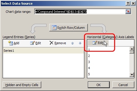
In the Select Data Source dialog, the chart data range (the cells containing the data that is being charted) is given near the top. To change the horizontal axis labels, click the Edit button in the Horizontal Axis Labels section of the dialog:
When the Axis Labels dialog appears, go to your worksheet and highlight the column that contains the end of period values. The range of cells that you select will become the Axis label range as shown here:
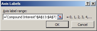
Click the OK button to close the Axis Labels dialog and then click the OK button to close the Select Data Source dialog.
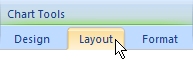
c) Go to the Layout Tab
The next step is to set the chart title. With the chart active, click the Layout tab in the chart tools section:
d) Set the Chart Title
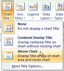
In the Labels section, select the Chart Title tool button and then the Above Chart option as shown below. Excel will add a default chart title but you should change the title to "Savings Account Balance".
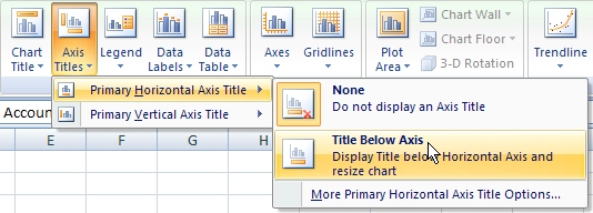
e) Set the Horizontal Axis Title
In a similar fashion, we will set the horizontal axis title to "Months". Still in the Labels section, select the Axis Titles tool, the Primary Horizontal Axis Title option, and the Title Below Axis option. Then, type in the word "Months" and tap the Enter key.
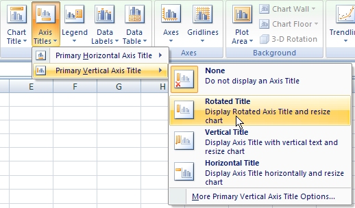
f) Set the Vertical Axis Title
Set the y-axis title to "Balance". Select the Axis Titles tool, the Primary Vertical Axis option, and the Rotated Title option. Then type in the word "Balance" and tap the Enter key.
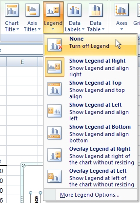
g) Delete the Legend
Since we are charting only one set of data, our chart does not need a legend. Select the Legend tool (in the Labels section) and the None option:
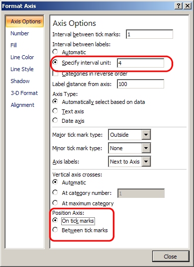
h) Format the Horizontal Axis
On the x-axis, set the number of intervals between labels to four and position the axis on the tick marks. Click the Axes button. Then, click the Primary Horizontal Axis button. Then, click the More Primary Horizontal Axis Options button.
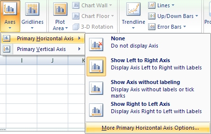
Set the interval unit to 4 and check the "on tick marks" button as illustrated below:
The interval unit should be set so that the x-axis labels are not all crowded together. The exact value depends on the size of the chart and the number of periods. In general, the larger the number of periods, the greater the interval unit. Positioning the axis on tick marks means that the y-axis will cross the x-axis exactly at period zero (the beginning of the investment). You should always select this option for line graphs.
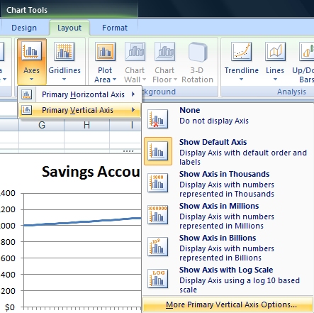
i) Format the Vertical Axis
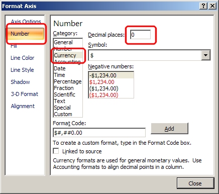
Change the number format of the y-axis to currency with a dollar sign symbol and zero decimal places. Click the Axes button. Then, click the Primary Vertical Axis button. Then, click the More Primary Vertical Axis Options button.
In the Format Axis dialog, select the Number option, select the currency format, and set the number of decimal places to zero:
Your final chart should look something like this:
8. Save your workbook.
You can check your work by looking at my workbook: Lab01Done.xlsx
The primary advantage of using cell references in Excel formulas is that you can alter problem parameters and Excel will recalculate all of the cell values automatically.
1. Change the present value to $1.00 and the term to one year. Move to the cell that shows the total interest (cell B10) and increase the number of decimal places. You'll see that the interest on $1.00 for one year is about 0.0407 dollars or 4.07%. Reduce the number of decimal places back to two.
The interest on one dollar for one year, expressed as a percent, is the effective rate or the annual percentage yield (APY). The APY is a true indicator of how much interest you are earning because it takes into account the effect of compounding. The nominal annual rate is not a true indicator because it does not take the effect of compounding into account. That is why it is called the nominal rate.
2. Change the present value to $10,000 and the years back to 5. The formula results for future value and total interest should change to $12,209.97 and $2,209.97 respectively. However, the results given by the table will be 12,210.01 and 2,210.01 respectively. Remember that the formulas do not take rounding into account and, as a result, yield only very good approximations to the actual values.
3. Change the interest rate to 6.00%. The formula results become $13,488.50 and $3,488.50. The table results become 13,488.47 and 3,488.47.
4. Change the periods per year to 4 and the number of years to 15. The total number of periods should still be 60. The formula results should be $24,432.20 and $14,432.20. The table results will be $24,432.15 and $14,432.15.
Any of the basic parameters (P, r, t, ppy) can be changed freely and the formula results will change accordingly. However, since our table was based on exactly 60 periods, it will only be correct if the number of periods is 60.
Excel provides a function named FV that can be used to calculate the future value of a one-time investment:
=FV(rate, nper, pmt, [pv], [type])
where
The pmt and type arguments are used to find the future value of an annuity which we haven't got to yet. For now, we will set each of these arguments to zero. Like the TVM Solver, cash outflows are indicated by negative values and cash inflows are positive. As a result, the present value should be entered as a negative value (since it represents a cash outflow).
In cell B9, use the FV function to find the future value of this investment using cell references for rate, nper, and pv. Help
The lab exercise is NOT a group project. You are to complete this assignment by yourself with no help from others.
The lab exercise is to be completed on the worksheet named "Lab Exercise". The names of the worksheets are on the tabs at the bottom of the Excel Window.
How much would you have to invest at 5.2% compounded quarterly if you wanted to have $10,000 at the end of five years? Generate a line chart that illustrates the growth of this investment over the five year term.
You can use the same basic layout as you used in the example above. In this exercise, however, the future value is given and you will need to implement the present value formula to find the present value (or use Excel's PV function).
The exponentiation operator in Excel is the caret (^). To enter a negative exponent in Excel, just enter a hyphen in front of the cell reference. For example, to raise the contents of cell C1 to the negative of the value in cell C2 you would use this formula:
=C1^-C2
Submit the lab exercise by saving your Excel file and sending it to me as an email attachment. Your grade will be based on the correctness of your results, the use of proper techniques, and the appearance of your work. That is, it should not only be correct but it should also look nice.