
When the possible outcomes of an action all have exactly the same probability, we say that the action has equally likely outcomes. When flipping a coin, heads or tails is equally likely (each has a probability of 1/2). When an ordinary die is rolled, the six possible outcomes are equally likely (each has a probability of 1/6).
The act of rolling a pair of dice results in 36 equally likely outcomes (using the fundamental counting principle: 6 * 6 = 36). Even though these 36 outcomes are equally likely, the probabilities for different dot sums are not since a dot sum is an event and the number of successful outcomes varies with the dot sum.
In this lab exercise, you will simulate experiments based on actions that have equally likely outcomes. In the next lab exercise, you will simulate experiments involving actions that do not have equally likely outcomes.
If you haven't already done so, you'll need to read the material on computer simulation.
To simulate the outcome of an action with equally likely outcomes, we need to generate a random integer value within the range of values used to represent the possible outcomes. The Excel expression below will generate a random integer value within a sequence of n consecutive integer values in the range A to B (inclusive):
RANDBETWEEN(A,B)
The table below provides some specific examples.
| Range of Consecutive Integer Values | Excel Expression |
| 1, 2, 3, 4 | RANDBETWEEN(1,4) |
| 10, 11, 12, 13 | RANDBETWEEN(10,13) |
| 3, 4, 5, 6, 7, 8, 9 | RANDBETWEEN(3,9) |
In this exercise you will simulate an experiment that consists of rolling an ordinary die 60 times and tabulating the corresponding empirical probabilities for the possible outcomes (1 to 6, inclusive). Finally, you will calculate the theoretical probabilities and generate a chart that compares the empirical and theoretical probabilities.
1. Download and open the file, Lab08.xlsx. Remind me how. Put your name in cell B1 of the one die worksheet.
2. Click on the tab labeled "One Die" and enter your name in cell D1.
3. Using the general formula given in the preceding section, determine the formula for randomly generating an integer value in the range 1 to 6. Enter your formula in cell A5 and use the fill handle to copy it into cells A5:A64. This will simulate sixty trials of this experiment. Are all of your values between 1 and 6? If not, correct your formula and try again. Help
4. In the column labeled "Dots", I have listed the possible outcomes for each trial of this experiment. In the frequency column you want to "count" how many times each corresponding outcome has occurred. That is, you want to count the number of ones, the number of twos, and so on. Excel provides a convenient way for doing this:
=COUNTIF(range, criterion)
This function returns the number of cells within the specified range of cells that meets the given criterion. In this case, the range is A5:A64 because these cells contain the results of our simulated experiment. For each row in the frequency column, the criterion is the corresponding outcome in the outcome column. Enter the formula shown below into cell D5. This formula counts the occurrences of the value in cell C5 (the number of 1's) appearing in the range of cells A5:A64 (our simulated die rolls).
=COUNTIF(A$5:A$64, C5)
Notice the use of the $ in the range addresses. When a formula is copied in Excel all of the cell addresses are adjusted relative to the new location. For example, copying the formula down to the next row would normally cause the range to become A6:A66 and the criterion reference to become C6. The criterion reference is correct but the range references would be wrong. The dollar signs in the formula make the row references absolute so they will not change as the formula is copied down the column.
5. Copy the formula in cell D5 into the range of cells D5:D10
6. Click on cell D11 (the first cell below the observed frequencies) and use
the AutoSum tool button ( Σ ) to find the sum of the frequencies. The sum should be 60, the number of trials. If it doesn't,
you have made a mistake somewhere.
![]()
7. Recall that the empirical probability of a specific outcome is calculated by dividing the observed frequency of that outcome (in the frequency column) by the number of trials (the sum you calculated in the previous step). Enter the appropriate formula in cell E5 (being careful about absolute and relative references), copy it into cells E5-E10, and set the number of decimal places to three. (Remember that as you perform these actions, the frequencies will change because the die "rolls" are being recalculated.) Help
8. The theoretical probabilities are all 1/6. Enter the formula
"=1/6" in cell F5. Don't omit the equal sign!
![]()
If you forget the equal sign, Excel will think you are entering the date January 6. Even if you go back and correct the cell contents, Excel will still try to format the cell as a date. To change the format back to numeric, you will have to right-click on the cell, click on the Format Cells option, select the Number tab, and click on "Number" in the category list.
9. For a single die, the theoretical probabilities are all the same. Each possible outcome has a theoretical probability of 1/6. Therefore, copy the formula you just entered in cell F5 into cells F5:F10 and set the number of decimal places to three.
10. Highlight cells E11:F11 (the cells immediately below the probability columns) and click the AutoSum tool button ( Σ ). Both totals should be exactly one.
11. Format cells D10:F10 with a heavy bottom border. Center the values in cells D11:F11. Your final table should look something like this (your empirical probabilities will be different):
The basic steps for creating a graph are the same as you learned in the finance labs at the beginning of the semester.
1. Highlight the columns containing the empirical and theoretical probabilities including the column headings (E4:F10). Do not include the totals.
2. Click the Insert tab:

3. Click the column chart button and insert a clustered column chart (this is the first type in the list).

4. Click the Select Data button to use the value in the Outcome column as the horizontal axis labels.
5. Click on the Layout tab:

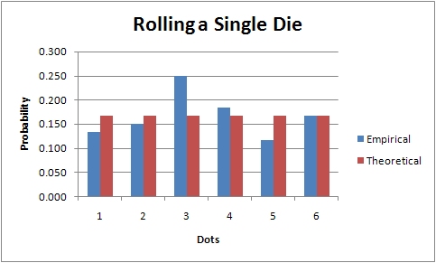
6. Using the appropriate tools set the chart title to "Rolling a Single Die", the horizontal axis title to "Dots", and the vertical axis title to "Probability". Your graph should look something like the one below (though your bar heights may differ from mine).
You can check your work by looking at my workbook.
When rolling a pair of dice the dot sum is found by adding the outcome of the first die to the outcome of the second die. When simulating the rolling of two dice you must follow the same procedure. You must add together two expressions; each of which generates a random number between 1 and 6. The first expression simulates the first die and the second expression simulates the second die. Adding them together gives the dot sum.
1. Click on the "Two Dice" tab and enter your name in cell D1.
2. Figure out the formula you would use to simulate the rolling of a pair of dice. To see if you got it correct, follow this link to the correct formula.
3. Enter the formula into cell A5 and copy it into cells A5:A604 to simulate 600 rolls.
4. In cell D5, enter a formula (using the COUNTIF function) to count the number of times a dot sum of 2 was observed. Copy your formula into cells D5:D15. Use the AutoSum tool button to find the total of the observed frequencies and make sure you get a value of 600.
5. Enter the formula for the empirical probability in cell E5 being careful about relative and absolute references. Copy the formula down the column by dragging the fill handle.
6. On a piece of paper, create the sample space for rolling a pair of dice (as we did in class).
7. For each possible dot sum, enter the theoretical probability in the theoretical probability column. Be careful, the probabilities for the various events (dot sums) are not all the same. Also, don't forget to include the equal sign when you enter a theoretical probability or Excel will think you are entering a date.
8. Highlight cells E16:F16 and use the AutoSum tool button to calculate the column totals. Make sure that both totals are exactly one.
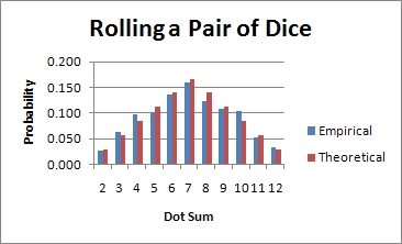
9. Generate a chart illustrating the empirical and theoretical probabilities.
When you are all done, your chart should look something like this:
You can check your work by looking at my workbook.
Each trial of an experiment consists of flipping three coins and counting the number of heads. The least number of heads is 0 and the greatest number of heads is 3.
1. Click on the "Three Coins" tab and enter your name in cell D1.
2. Since a coin has only two possible outcomes and you are recording the number of heads, you can let the value zero represent a tail and the value one represent a head. Each coin is represented by an expression that yields a random value in the range 0 to 1. Since you want to simulate three coins you will need to add three of these expressions together with the sum representing the number of heads. Make your best effort to derive the appropriate formula and then follow this link to see my formula.
3. Enter the correct formula in cell A5 and copy it down the column into 100 cells. Verify that all of these cells contain a value between zero and three!
4. Enter a formula using "COUNTIF" in cell D5 to count the number of times the outcome was zero heads. Use absolute references where appropriate.
5. Copy your formula into the remaining cells in the frequency column. Use the AutoSum tool button to find the sum of these frequencies and verify that you get a value of 100. Remember that the number of trials (n) should always equal the sum of the frequencies.
6. Enter the appropriate formula for the empirical probability of getting no heads in cell E5 and copy it down the column. Don't forget to use absolute references when necessary.
7. On a piece of paper, generate the sample space for flipping three coins and determine the theoretical probabilities (leave them as fractions).
8. Enter the theoretical probabilities in the theoretical probability column. Don't forget to begin each entry with an equal sign.
9. Make sure that the sums of the empirical and the theoretical probabilities are both exactly one.
10. Create a chart comparing the empirical and theoretical probabilities.
You can check your work by looking at my workbook.
Remember those childhood games that had spinners and how you'd argue whether the spinner was on the line or not? Let's pretend that you have a more complicated game that requires you to add two spinner values together. The first spinner is evenly divided into regions numbered 1 to 4 and the second spinner is evenly divided into regions numbered 6 to 10.
1. Click on the "SPINNER" tab and enter your name in cell D1.
2. Under the column labeled "Sum" enter the possible values that could be generated by spinning the two spinners and adding the results. List the values in ascending order.
3. Create an expression that will generate a random value between 1 and 4 and a second expression that will generate a random value between 6 and 10. In cell A5, enter a formula that will add these two expressions together to simulate adding the outcomes from these two spinners. Copy your formula down into 200 cells.
4. Enter the appropriate COUNTIF formula in the first cell of the frequency column and copy it down the column. Find the sum of the frequencies and verify that it is 200.
5. Enter the formula for empirical probability in the first cell of the empirical probability column and copy it down the column.
6. On a piece of paper, find the sample space (much as you did for the two dice) and use it to determine the theoretical probabilities.
7. Make sure that the sum of the values in each probability column is exactly one.
8. Finally, create a chart comparing the empirical and theoretical probabilities.