

The simplex method is an algebraic algorithm for solving linear maximization problems. Beginning at the origin, this algorithm moves from one vertex of the feasible region to an adjacent vertex in such a way that the value of the objective function either increases or stays the same; it never decreases. This movement continues until the vertex that yields the optimal solution is reached.
We will use the example below to demonstrate how and why the simplex method works. This is the same example used on the geometric introduction to linear programming page.
A manufacturer of lightweight mountain tents makes a standard model and an expedition model for national distribution. Each standard tent requires 1 labor-hour from the cutting department and 3 labor-hours from the assembly department. Each expedition tent requires 2 labor-hours from the cutting department and 4 labor-hours from the assembly department. The maximum labor-hours available per day in the cutting department and the assembly department are 32 and 84 respectively. If the company makes a profit of $50 on each standard tent and $80 on each expedition tent, how many tents of each type should be manufactured each day to maximize the total daily profit (assuming that all tents can be sold)?
Here is the mathematical model for this problem:

In the simplex method, each inequality constraint is written as an equation by introducing a slack variable. The cutting constraint inequality is written as an equation by introducing the slack variable s1:
x1 + 2x2 ≤ 32 becomes x1 + 2x2 + s1 = 32
The value of the slack variable s1 represents the number of labor-hours that are available for cutting tents but that are not used. For example, suppose 10 tents of each type are manufactured each day. The number of labor-hours required to cut 10 standard tents (at 1 hour per tent) is 10 hours and the number of labor-hours required to cut 10 expedition tents (at 2 hours per tent) is 20 hours for a total of 30 hours which is 2 hours less than the 32 labor-hours available for the cutting operation. These 2 available, but unused, labor-hours represent the slack and the value of s1 would be 2 labor-hours. Given the original constraint (x1 + 2x2 ≤ 32) we know that s1 ≥ 0. (This is true for all slack variables)
In a similar fashion, the second inequality can be written as an equation by introducing a second slack variable, s2, whose value represents the number of labor-hours available for the assembly operation but that are not used:
3x1 + 4x2 ≤ 84 becomes 3x1 + 4x2 + s2 = 84
If 10 tents of each type are manufactured, the number of labor-hours required to assemble the standard tents (at 3 hours per tent) is 30 and the number of labor-hours required to assemble the expedition tents (at 4 hours per tent) is 40 for a total of 70 labor-hours which is 14 hours less than the 84 labor-hours available for the assembly operation. In this case, then, the value of s2 would be 14 labor-hours.
Finally, the objective function is written in the same form as the new constraint equations (with the variables on the left and a constant term on the right):
P = 50x1 + 80x2 becomes -50x1 - 80x2 + P = 0
Putting all the pieces together, the alternate mathematical model becomes:
   x1 +  2x2 + s1            = 32  « Cutting Constraint
  3x1 +  4x2      + s2       = 84  « Assembly Constraint
-50x1 - 80x2           + P   =  0  « Objective Function
   x1, x2, s1, s2 ≥ 0              « Non-negative Constraints
In this alternate mathematical model, the variables can be divided into two mutually exclusive groups (basic and non-basic) with the restriction that there always as many basic variables as there are equations. In each case, the non-basic variables are set to zero and the corresponding values of the basic variables are then calculated. These values represent a basic solution. If all of the values in a basic solution satisfy the non-negative constraints, it is a feasible basic solution. If a maximization problem has a solution at all, it will be at one (or possibly more) of these feasible basic solutions.
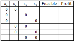
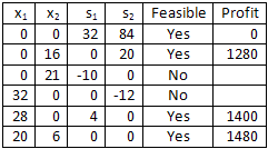
In the table below, I have demonstrated how the four variables in our model can be divided into basic and non-basic variables in six different ways. You can identify the non-basic variables by the fact that they have been set to zero.
Next, we solve for the values of the basic variables (using the constraint equations in the alternate mathematical model above). The results are shown in the table below. Notice that, for each basic solution, the ordered pair (x1, x2) is the intersection of two lines in the graphical representation of this problem.
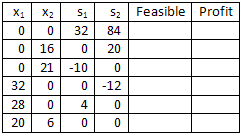
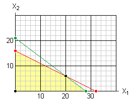
You should also notice that not all of the basic solutions are feasible solutions. Any solution in which the value of a variable is negative is not a feasible solution since it violates at least one of the non-negative constraints. Consequently, the middle two basic solutions are not feasible. Note that the feasible solutions correspond to the vertices of the feasible region.
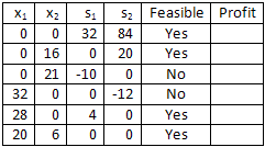
Finally, we can calculate the profit for each feasible solution in order to determine which solution generates the most profit. The maximum daily profit is $1,480 when the company manufactures 20 standard tents and 6 expedition tents per day.
The approach taken in the previous section works well enough with very simple problems but doesn't scale well to larger, more difficult, problems. The simplex method is an algebraic algorithm that allows us to arrive at the same result without the need for a graphical representation of the problem nor the need to determine any of the feasible solutions. In essence, it begins at the feasible solution at the origin and generates additional feasible solutions such that each successive solution is at least as good as the previous solution and usually better. The algorithm terminates when the optimal solution has been reached.
The algorithm begins with a matrix representation of the alternate mathematical model as shown here:

This is the initial tableau. The column headings are to remind us of which variable is associated with the coefficients in the column.
Each tableau represents a feasible basic solution. The row headings in a tableau indicate the basic variables (s1 and s2, in this initial tableau) and the objective function (P). The remaining variables (x1 and x2, in this case) are non-basic variables. As noted above, the non-basic variables in any basic solution have a value of 0. Consequently, x1 = 0 and x2 = 0 and our alternate mathematical model becomes:
    0 +  2∙0 + s1            = 32  « Cutting Constraint
  3∙0 +  4∙0      + s2       = 84  « Assembly Constraint
-50∙0 - 80∙0           + P   =  0  « Objective Function
or, ignoring the zero terms:
               s1            = 32  « Cutting Constraint
                    s2       = 84  « Assembly Constraint
                         P   =  0  « Objective Function
Notice that these values for the basic variables and the value of the profit can be found in the right-most column of the initial tableau. This is true for each tableau generated by the simplex method.
The pivot operation transforms a given tableau into a new tableau that represents a different feasible basic solution for which the value of the objective function is greater than or equal to the previous value. Consequently, each pivot operation results in a feasible solution that is closer to the optimal solution.
The pivot column corresponds to the most influential variable; the variable that has the greatest ability to increase the value of the objective function. In our example, each standard tent increases the profit by $50 but each expedition tent increases the profit by $80. Consequently, the more influential variable is the number of expedition tents. In the tableau, the coefficients of the objective function are negative so the pivot column is the column in which the most negative value appears in the bottom row (the row that corresponds to the objective function):

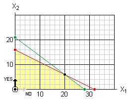
Let's take a closer look at what we are doing by choosing the pivot column. As noted earlier, the initial tableau represents the feasible basic solution at the origin; the lower-left corner of the feasible region. From there we can either move to the right (increase x1) or move up (increase x2) as illustrated here:
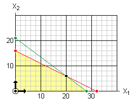
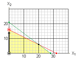
The algorithm chooses the direction based on the most influential variable. As noted above, manufacturing one expedition tent has a greater impact on the profit than manufacturing one standard tent. Consequently, the algorithm chooses to move up (to increase the number of expedition tents):
For each row that corresponds to a basic variable and that has a positive value in the pivot column, find the quotient you get if you divide the constant term (in the right-most column) by the value in the pivot column. The pivot row is the row that yields the smallest quotient. All of the rows except the bottom row correspond to basic variables. In our example, both of these rows have a positive value in the pivot column. In the first row, the quotient is 32/2 = 16. In the second row, the quotient is 84/4 = 21. Consequently, the first row is the pivot row (because its quotient was smallest):

This process appears somewhat arbitrary so let's take a closer look. We have already seen that choosing the pivot column means we will move up to find our next basic solution. As you can see in the picture below, there are two basic solutions in that direction but only one of them (the lower one) is feasible. This technique for choosing the pivot row moves us to the next feasible basic solution (in the desired direction).
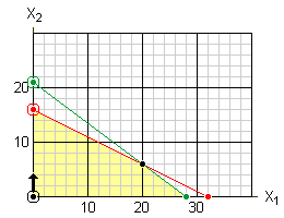
Solve the equation of the red line (which corresponds to the cutting constraint) for x2:
x1 + 2x2 = 32
     2x2 = - x1 + 32
      x2 = - x1/2 + 32/2 <== The quotient
      x2 = - x1/2 + 16
This is the slope-intercept form of the equation of the line and indicates that the line crosses the x2 axis at 16.
Similarly, solve the equation of the green line (which corresponds to the assembly constraint) for x2:
3x1 + 4x2 = 84
      4x2 = -3x1 + 84
       x2 = -3x1/4 + 84/4 <== The quotient
       x2 = -3x1/4 + 21
From this equation, we can readily see that the green line crosses the x2 axis at 21.
In effect, the quotient obtained by dividing the constant term in a given row by the value in the pivot column is the distance from the current basic solution to another basic solution measured in the direction of the pivot column axis. By selecting the row with the smallest quotient, the algorithm selects the closest of these basic solutions which will always be another feasible solution:
The pivot element is the element at the intersection of the pivot column and the pivot row. In our initial tableau, the pivot element is 2:

The pivot operation transforms the tableau for the current solution into the tableau that corresponds to the next solution. The variable corresponding to the pivot column (the entering variable) replaces the variable that corresponds to the pivot row (the exiting variable) in the list of basic variables (the row headings). The process is basically the same as that used in solving a system of linear equations using Gaussian elimination. Using row operations, set the pivot element to 1 and all other values in the pivot column to 0. Applying the operations
Replace Row1 with 0.5*Row1
Replace Row2 with  -4*Row1 + Row2
Replace Row3 with  80*Row1 + Row3
results in this new tableau where variable x2 replaces s1 in the list of basic variables:

The row operations indicated above can be done using your TI-83 calculator.
You'll notice that this solution corresponds to the upper-most vertex of the feasible region.
![]()
![]()
![]() [B]
[B]
I saved the initial tableaux as matrix A so it is safe to save the answer after the first pivot operation as matrix B. You want to save your work because if you use your calculator for anything else, such as finding the quotients in the next step, you will have to start the matrix operations all over again from the beginning.
Since there is a negative value in the bottom row of this new tableau, we are not done and must repeat the whole process again.
Since we just finished dealing with the number of expedition tents, the only thing we can do now to increase the profit is to increase the number of standard tents. This is reflected by the fact that the only column with a negative value in the bottom row is the x1 column which becomes the pivot column:

Again, it helps to look at this graphically. In the illustration below, we want to move from our current solution to another, better solution. We can either move straight down or along the red line. Moving down is counterproductive since it leads right back to where we started. Consequently, the only real option is to move along the red line towards the basic solutions in that direction.
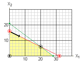
The slope (Δx2/Δx1) of the red line is -1/2. Consequently for every two additional standard tents we make, we must reduce the number of expedition tents by 1. Our profit will increase $100 for those 2 additional standard tents but will decrease by $80 for the expedition tent we can no longer make. Consequently, the net change in the profit is $20 for every 2 standard tents or $10 per tent. This is reflected by the value -10 in the bottom of the pivot column.
The second row is the pivot row since 20/1 = 20 is less than 16/0.5 = 32.

These quotients represent the distance (parallel to the x1 axis) to the two basic solutions along the red line. Only the first solution is feasible (x1 = 20). The second solution (x1 = 32) is not feasible. Notice once again that this process of selecting, as the pivot row, the row with the smallest quotient, moves us to the next feasible solution in the desired direction.
Since the pivot element is already 1, all we need to do is perform row operations that will make the remaining values in the pivot column equal to 0. Applying the operations
Replace Row1 with  -0.5*Row2 + Row1
Replace Row3 with  10*Row2 + Row3
results in this new tableau where variable x1 replaces s2 in the list of basic variables:

The row operations indicated above can be done using your TI-83 calculator.
This represents the optimal solution since there are no negative terms in the bottom row. The maximum profit of $1,480 a day can be made by manufacturing 20 standard tents and 6 expedition tents each day. The graphic below illustrates the path that we have taken from the origin to the optimal solution.
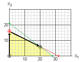
This production schedule fully utilizes the number of hours for both cutting and assembly since both slack variables have a value of 0.